Introduction

Because traffic data provide quantitative measurements of the intensity and quantity of communication between the entities (predominantly users and servers) which share access to a network, we should be able to estimate social network behaviour from traffic samples (trace files). The key difference between social network behaviour, as an interpretation of traffic, vs traditional traffic theory, is that it emphasizes end-to-end patterns, rather than traffic behaviour over time. For example, in traditional traffic theory, it is conventional to view a flow as equivalent, or a generalization, of a TCP flow. Thus, it has a start and an end. But in the analyses undertaken here, the start and end are not considered important. All the traffic between a certain originating IP address and a different destination IP address are viewed as a flow.

Social network behaviour is about who is talking to who, how much they are saying, and the patterns within these conversations. There are many potential patterns, so we need to focus on certain key patterns initially, for example, whether there exist groups of correlated sources, or of destinations, or of O-D flows. For reasons of privacy, the true identity of the users represented in a traffic trace is not normally available. In any case, the term social network behaviour is not used to refer to the identification of specific connections or relationships between users. In this paper social network behaviour is defined to mean statistical characteristics which result from the variation in connection and quantity of communication between the members of a community. An example of social networking behaviour which might be expected, and which is discovered in the traffic traces in this study, is the heavy-tailed character of the distribution of the total traffic between each origin-destination pair (O-D pair); that is to say: a small number of O-D pairs carry a large quantity of traffic, and a large number of O-D pairs carry relatively little traffic. This heavy-tailed behaviour is not just observed to occur, but its specific ?shape? can, and has been, estimated.

We seek to interpret the traffic, even on one link, as a guide to the behaviour of the whole network. If the observed link is in the core network, the range of IP addresses which appear on it will be very large, and although the traffic observed is a sample, because the features being observed are of a statistical character, rather than concerned with specific user identities, there is no obvious reason for the use of a sample to cause the estimates obtained to be biassed.

Why social behaviour is important

Given the importance of modelling the traffic matrix (TM) for number of network aspects, good models of traffic matrices are important. The paper (Erramill, Crovella, & Taft, 2006) is concerned with the paucity of studies which are focused on complete models for TM, despite the importance of TM modelling. Traffic modelling and analysis is an essential preliminary step in network design and management. A number of point-to-point traffic models which have been studied in the literature are discussed in (Chandrasekaran, 2009), (Vardi, 1996). However, there is much less work currently available on models of all the traffic on a network.

In order to develop QoS architecture within the Internet networks, a strong traffic model is required for accurate performance evaluation and traffic analyses (Adas, 1997). What is needed is not only a model for the traffic on each link, but a model for the traffic of the whole network (Lakhina et al., 2004). This is the type of model we seek in this paper.

A whole network traffic model will enable to us to see a clear picture for the behaviour of traffic which is statistically sound. Whole network traffic analysis is difficult because the number of origins, destinations, and origin-destination pairs which arise may be so large that naive methods of analysis may fail, or the time taken to produce a result may take too long. In some cases there may be more than 1 million distinct sources, destinations, or O-D pairs referenced in a sample. On the other hand, in our analysis it may be necessary to identify correlations between different origins, or destinations, or O-D pairs, which will not be possible without some carefully designed algorithms.

To gain a better understanding of whole-of-network traffic it is useful to focus on origin-destination flows (O-D flows). We need to compare and contrast different origins, different destinations, and different O-D flows. This analysis needs to be statistical in its framework, and if possible we would like to identify the key statistical features which explain network behaviour in terms of origins, destinations, and O-D flows.

Source of data

In this paper, traffic data from Center for Applied Internet Data Analysis(CAIDA) (Center for Applied Internet Data Analysis, 2016) is analysed by a variety of methods to discover features of the social network from which the traffic is generated. The IP addresses in CAIDA datasets are anonymized. The Crypto-PAn tool was used to anonymize the IP addresses in the dataset. Crypto-PAn is a cryptography-based sanitization tool for network trace owners to anonymize the IP addresses in their traces in a prefix-preserving manner (Fan, Xu, Ammar, & Moon, 2004). This tool has the following properties: (a) the IP address anonymization is prefix-preserving. In other words, if two original IP addresses share a k-bit prefix, their anonymized mappings will also share a k-bit prefix; (b) the same IP address in different traces are anonymized to the same address, even though the traces might be sanitized separately at different time and/or at different locations.

Table 1 lists all the CAIDA datasets which are used in this paper. This table also contains the figures in which results from that particular data sets.

Summary of paper

In the next section, the traffic analysis methods are discussed. After this, the Antraff software is described. Followed by the description of a series of experiments that are discussed. Finally, the conclusion of overall work is presented.

Traffic Analysis Methods

Frequently used IP addresses

A traditional traffic matrix, which was used for many years in telecommunication networks, contains, for each origin-destination pair, the ?volume? of traffic (in Erlangs, or bits/sec), between the origin and the destination. By assigning a common column and row index to each node in the network, such data can be readily presented as a matrix. However, when monitoring Internet traffic, without complex processing to translate the IP addresses into node identities relative to a specific network, it may be difficult to identify the origin and destination nodes of packets. Using IP addresses in place of origins and destinations seems the logical step to overcome this problem, but the total number of IP addresses, even in IPv4, is too large to allow matrices with one row and column for each IP address.

For this reason, in order to analyse the traffic in a capture file such as those considered in this paper (The CAIDA UCSD Anonymized Internet Traces 2014 - [20140320], n.d.), an essential first step is to identify the frequently used IP addresses.

Finding the relatively small number of IP addresses which occur a significant number of times in a capture file has been achieved as follows:

The total number of distinct IPv4 addresses is approximately 4 billion, hence even though IP addresses are integers, we can?t use them as the indices of a vector or matrix. Even in quite a short traffic trace file, the total number of distinct IP addresses can easily exceed 1,000,000, and so it is not feasible to construct and manipulate vectors or matrices to describe the statistics of traffic from one IP address to another, even if this is precisely our objective.

So, instead, when matrices indexed by IP addresses are needed, instead of the IP address itself, as the index, we use its rank, and instead of including all IP addresses as potential indices, we only use the most important. IP addresses are all ranked, by their importance, measured as number of bytes sent from or to that address, and this rank is used both to select which IP addresses need to be included in the traffic matrix and the order in which they are included.

Traffic matrices

The simplest and traditional way to collect and manipulate traffic data is to create a matrix indexed by origins and destinations which contains the average bytes per second of the data from the origin to the destination, during the period of time considered. We will call this the mean traffic matrix. We can apply SVD to this matrix directly.

The mean traffic matrix can introduce some undesirable smoothing of the traffic. In particular, if the traffic is very bursty, the mean traffic matrix will not record this feature, and relying on it alone will lead to under-provisioning. We can avoid this by using a slightly different matrix. In this second approach, and the third, it is necessary to subdivide the traffic into time-slots during the analysis. The choice of time-slot length is significant, and will be varied. A typical value in the analyses presented here is 0.1 seconds.

When forming the second traffic matrix, which we term the variance matrix, the square of the bytes between each origin and destination, in each interval, is accumulated in each entry of the matrix, and divided by the interval length. We can also apply SVD to this matrix directly.

There are two variants of this type of matrix: if the mean-squared of the traffic in each interval is subtracted from the mean sum-of-squares, we arrive at the traditional variance, of the traffic passing between each origin and destination. However, it is also useful not to subtract the mean-squared. This matrix, which we could perhaps term the power matrix, includes the mean-squared, and hence is a better measure of the end-to-end load.

The third matrix type, which is the type used in (Lakhina et al., 2004) is formed by using O-D pairs, rather than origins and destinations, as the indices of the rows and columns. In each time-slot, the bytes delivered between each origin and destination are determined, and the product of entry C_ij in the covariance traffic matrix for this time-slot is the product of the bytes sent between O-D pair i and O-D pair j. These are then averaged over the trace to form the covariance traffic matrix.

Although these three traffic matrices may seem rather different, it turns out that they all reveal similar features of the traffic, and this will be explained in Subsection .

Principle Component Analysis and Singular Value Decomposition

Principal component analysis has been intensively studied and is widely in applied statistics. Principal component analysis (PCA) is a technique used to emphasize variation and bring out strong patterns in a new dataset. It?s often used to make data easy to explore and visualize. The paper (Ringberg, Soule, Rexford, & Diot, 2007) observed that PCA is the linear transform which retains the highest variance among all transforms reducing the data to a certain number of dimensions, for any choice for the number of dimensions. They used this property to argue that PCA is in some sense optimal, for the task of anomaly detection.

PCA is based on singular value decomposition, and in some cases a singular value decomposition of data (interpreted as a matrix) can be applied directly without first computing the covariance of the data.

In this case, the use of SVD is merely an alternative approach for producing the same analysis of the data into features. Singular value decomposition of a matrix is more general than PCA, which assumes the matrix being analysed is symmetric. On the other hand, the underlying optimality interpretation is still applicable, although in a generalised form, depending on the specific case.

The singular-value decompositions used in this paper all seek to identify features which summarise the traffic data as compactly as possible. This is a widely used methodology in many fields. Mathematically, a feature is a linear combination of the original data fields. Intuitively, a feature represents some recognisable characteristic of the data. For example, in data from photographs of faces, ?the nose? might be a feature discovered in the data in this way. The intuitive characteristics corresponding to the features discovered in the traffic data have not been identified in the literature applying SVD in this way (Lakhina et al., 2004), or by us, and it remains to be seen whether these intuitive characteristics will be discovered.

Antraff software

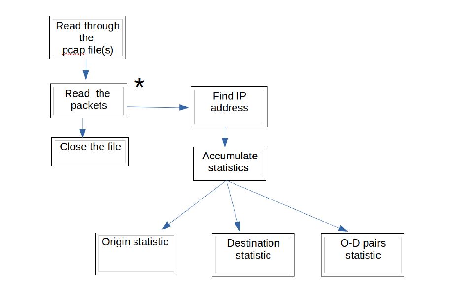
In order to carry out the analysis methods described above, and other methods, a software package called Antraff (Addie, 2016) has been developed. This software collects statistics of three different sorts:

(i)

Byte frequencies of origins, destinations, or O-D pairs. See Figure 1.

Figure 1: Algorithm for collecting origin/destination/O-D pair byte frequencies

(ii)

Accumulation of matrices of end-to-end traffic, followed by analysis of these matrices, by singular-value decomposition. There are three different ways in which traffic matrices can be accumulated, which can be intuitively described as mean, variance, and covariance matrices.

(iii)

Extraction of eigenflows associated with one of the three possible singular-value decompositions from the previous analysis method.

Volume statistics

The total number of origins, destinations, or O-D pairs in the pcap file or collection of pcap files being analysed may be more than we are able to store information about. However, it will be satisfactory if the only sources, destinations, or O-D pairs about which information is not collected are ones for which the total bytes, associated with this origin, destination, or pair, is small. By storing pointers to origins, destinations, or O-D pairs in a heap which is ordered so that the entity with the least total bytes, over an interval of time exceeding a certain threshold, can be easily removed, it is possible to identify origins, destinations, or O-D pairs which can be removed from the list of those about whom statistics are being collected without having to collect the information about this object, except for short periods of time. The volume information collected in this way is stored in such a way that we can estimate the distribution of bytes associated with each origin, destination, or O-D pair.

Eigenvalue statistics

The origin and destination statistics described in the preceding sub-subsection are used to identify the most important (in terms of numbers of bytes) origins, destination, and O-D pairs. Three types of traffic matrices are then estimated:

(i)

mean bytes, origin to destination;

(ii)

E(X²) and variance of bytes, origin to destination;

(iii)

covariance of O-D flows.

Note, the first two matrices are indexed by origin and destination IP addresses (not the actual IP addresses, but their rank), and the last of type is indexed by OD pairs (i.e. the rank of the OD pairs). Nevertheless, even in the last case, since each OD pair obviously also refers to an origin and a destination, the implications of all three matrices ultimately refer to a matrix which is indexed by origins and destinations.

Eigenflows

Once the singular decomposition of the traffic matrices outlined in the previous subsection has been completed it is possible to extract, from the traffic data, the eigenflows corresponding to each eigenvalue, and also the component O-D flows of each eigenflow. Each eigenflow is a linear-combination of O-D flows.

It is conceivable that there are highly important correlations between one O-D flow and another. For example, if a certain group of users engage in communication behaviour simultaneously, as a consequence of some shared activity of goal, this will lead to correlated O-D flows. The Antraff software is currently able to undertake singular value decomposition of traffic matrices and also extract both the eigenflows, and to display the O-D flows from which they are composed. However, it remains possible, at this stage, that the eigenflows are actually artificial, i.e. they are not actually a consequence of any genuine correlation between O-D flows.

Experiments

Source and Destination Byte Frequencies

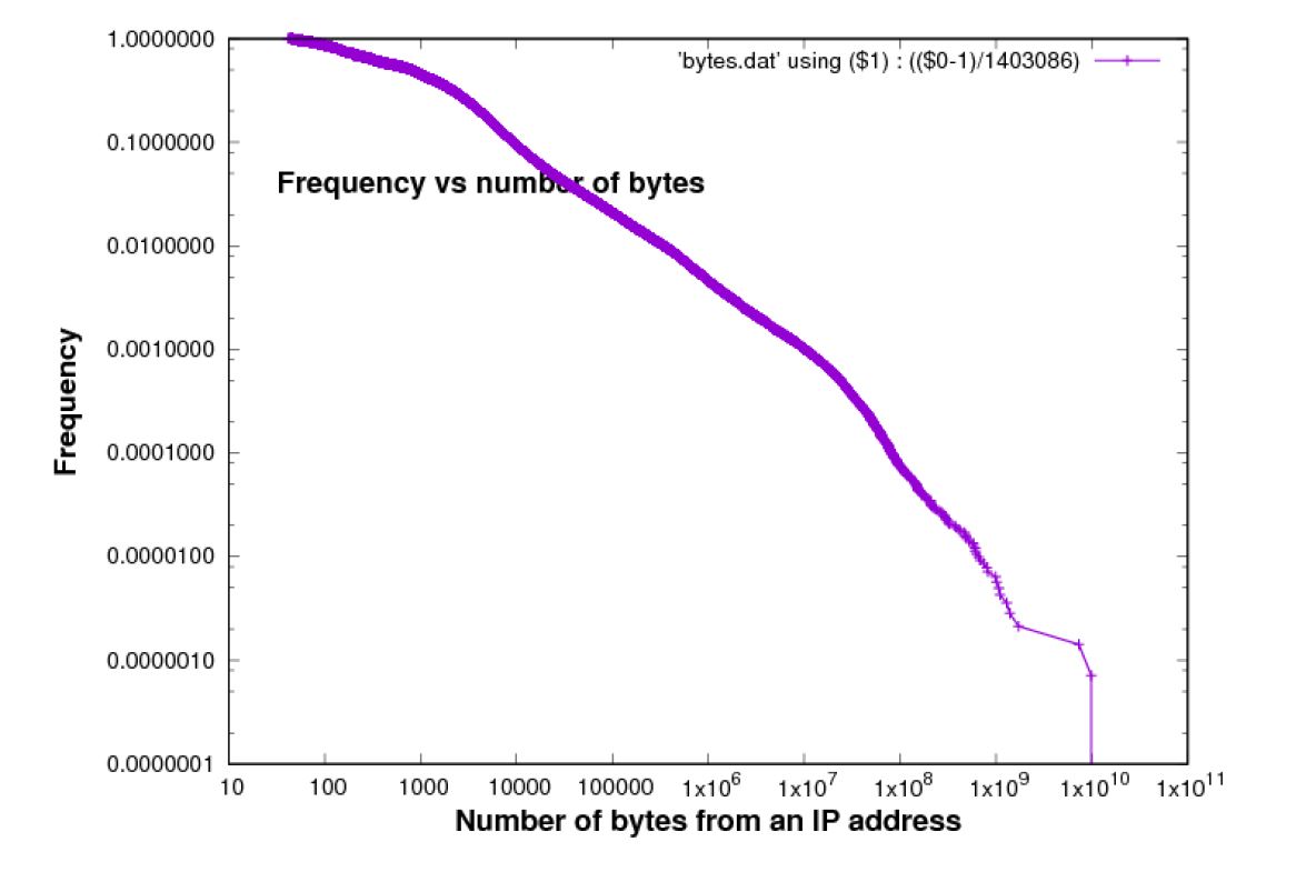
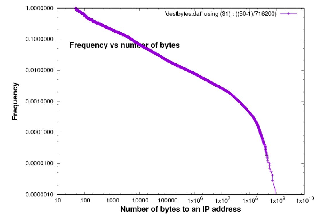
The traffic associated with individual IP addresses exhibits the Pareto principle, which is that a small proportion of IP addresses is associated with a high proportion of the traffic. In other words, the distribution of bytes per destination/source is heavy tailed. This is illustrated in Figures 2 and 3.

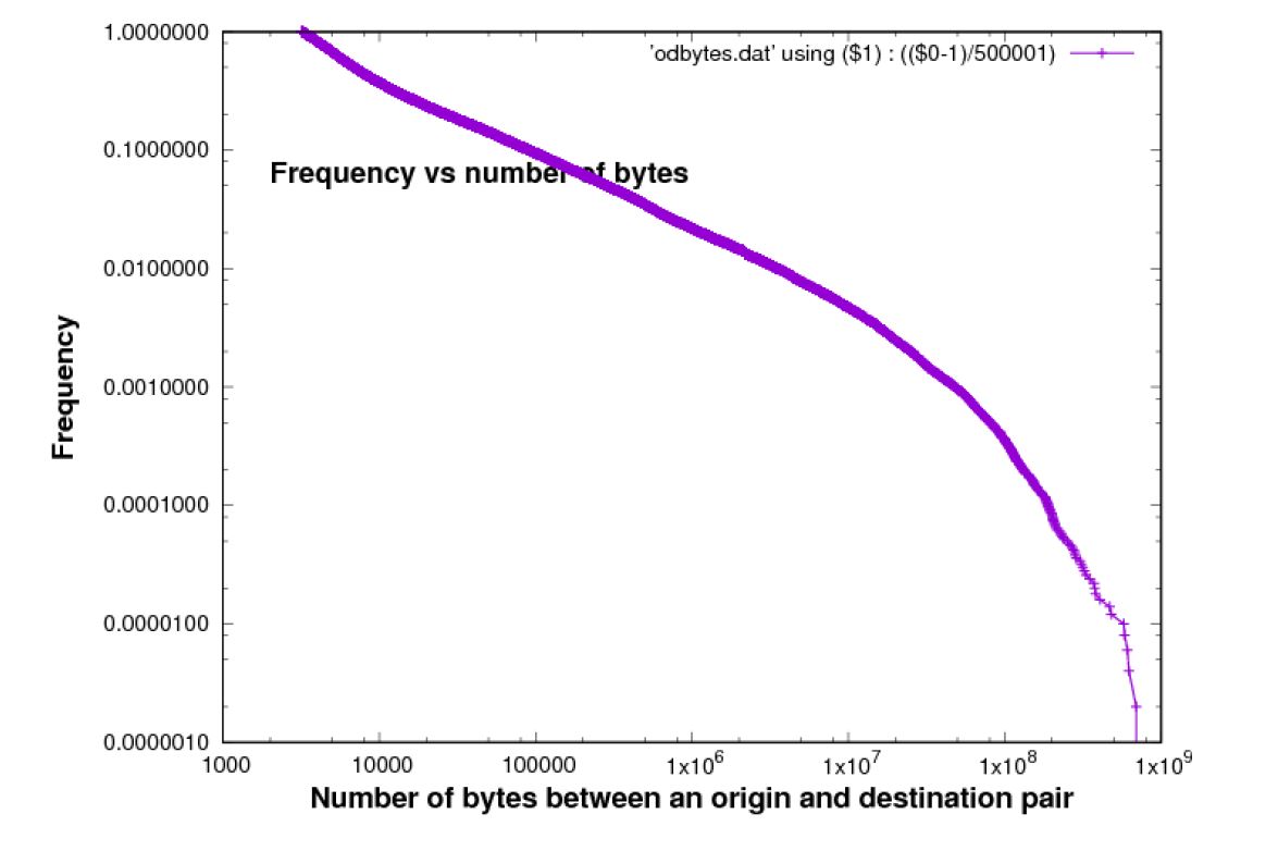
On a log-log scale, these plots are approximately linear. Both curves exhibit a tendency to ?roll off?, i.e. the curve falls away from the linear shape to the right. If the population was such that this plot was perfectly linear on a log-log scale, in a theoretical sense for the whole population, estimates of the curve from a finite sample will always exhibit this type of roll-off because of sampling error.

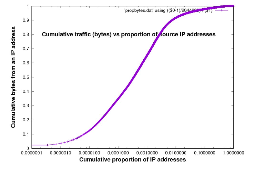
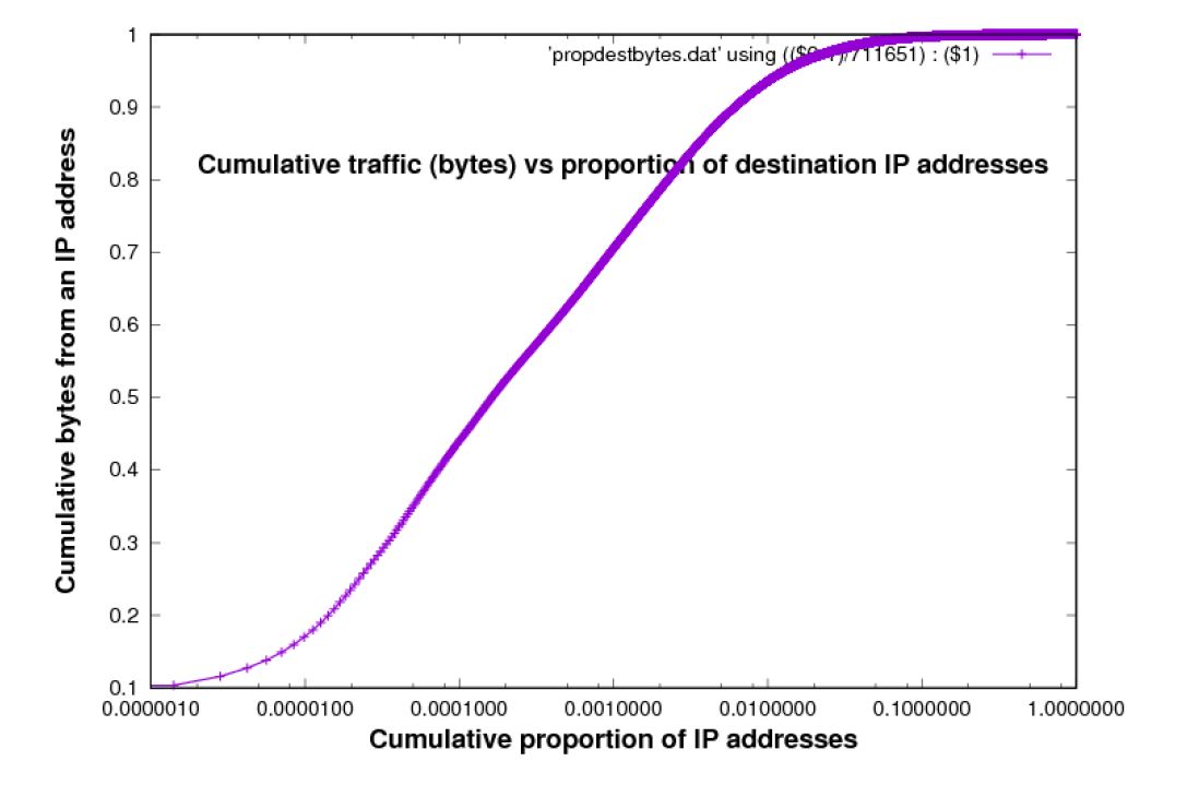
These Figures suggest that most bytes are accounted for by the larger sources of traffic. However we can?t actually read from these plots the proportion of bytes accounted by any initial portion (in decreasing weight) of sources. Figure 5 and 6 are designed to allow this. The Figures present the same information, but now the x-axis is the cumulative proportion of source and destination IP addresses respectively, in the data set, in order of weight, and the y-axis is the cumulative proportion of total bytes accounted for, by these IP addresses.

Figure 2: Bytes per source [Chicago 2015 data-set]

Figure 3: Bytes per destination [Chicago 2015 data-set]

Figure 4: Bytes per O-D pairs [Chicago 2015 data-set]

Table 1: CAIDA data-sets (each data set consists of 10 data files, as in Date/Time column, each file has same prefix and same suffix)

Figure 5: Cumulative sources bytes from an IP address vs Cumulative proportion of IP addresses [trace used: Chicago 2016 data-set]

Figure 6: Cumulative destination bytes to an IP address vs Cumulative proportion of IP addresses [trace used: Chicago 2015 data-set]

These Figures confirm the intuitive idea already introduced, that a small proportion of source IP addresses accounts for a large proportion of traffic, in bytes. However, the story is not extreme. To account for 90% of the bytes it is necessary to include at least 1% of sources, destinations, or O-D pairs, which is still quite a large number ? approximately 2,000 in for the traces used in Figures 5, 6 and 7.

O-D Pairs

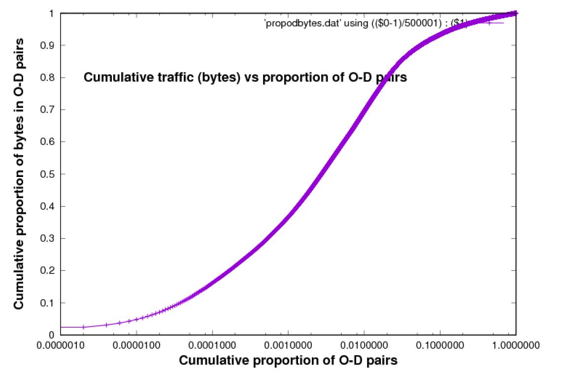
Figure 7: Cumulative bytes in O-D pairs address vs Cumulative proportion of O-D pairs [Chicago 2015 data-set]

Another way to analyse the traffic is shown in Figure 7. This time, instead of focussing on which sources or which destinations account for the traffic, it is the O-D pairs. We are looking here for an understanding of the structure of traffic from the point of view of O-D pairs which may prove to be very important in the development of an end-to-end traffic model.

The statistical results of O-D pairs, in this paper, are different from other studies in regard of the number of IP addresses which are analysed. The authors of (Lakhina et al., 2004) have analysed the structure of Origin-Destination traffic in a trace of Internet backbone traffic by using PCA to systematically decompose the structure of OD flow time series. They describe the trace the analyse as including hundreds of origins and destinations, and hundreds of flows. Another group of authors in (Susitaival, Juva, Peuhkuri, & Aalto, 2006) have analysed 1000 IP addresses to study the traffic characteristics of O-D pairs components, whereas the ones considered in this paper includes hundreds of thousands of origins and destinations, and millions of flows. Another difference is that the traces considered in this paper have durations of approximately one minute, whereas in (Lakhina et al., 2004) they consider traces lasting hours, days, or weeks. Figure 7illustrates the relation between cumulative bytes in O-D pairs vs cumulative proportion of O-D pairs starting with the largest flows because of the importance of these flows. This Figure shows that the first 10% of O-D pairs covers about 90% of bytes.

O-D-pairs vs origins and destinations

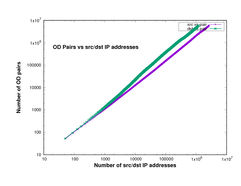
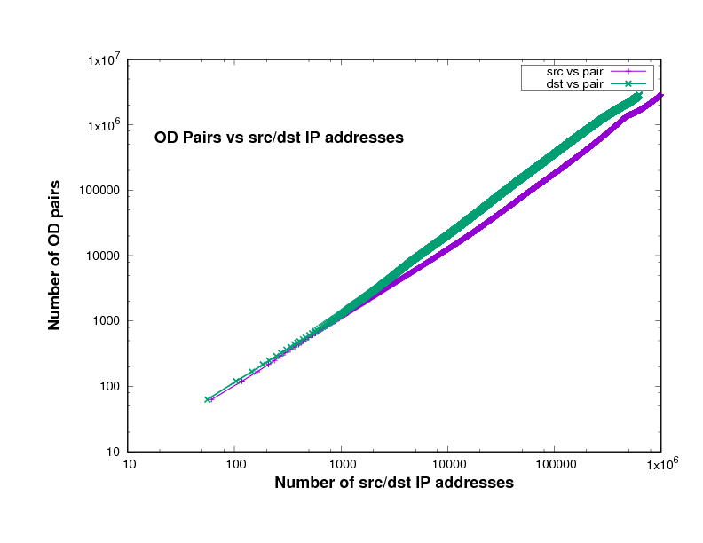
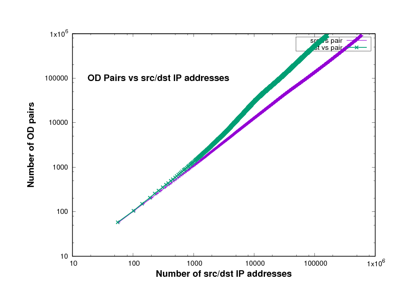
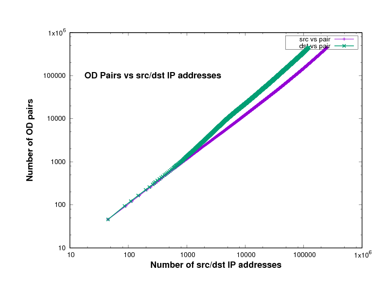
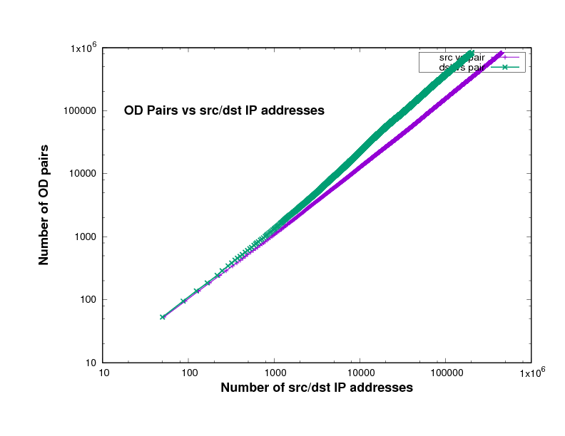
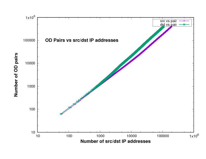
Figure 14 show the number of O-D pairs found in several files of different traffic traces a certain point in the file, against the total number of sources and destinations IP addresses. The traffic traces are captured from Chicago and San Jose on 2014, 2015 and 2016 in US. This has been plotted using log scales for both axes. The curve is approximately linear, with a slope close to 1. In fact the slope, in general on the log-log scale, means how broad is the community and it measures the diversity. This means that the value of the slope measures the breadth of the community whose communication is taking place in the trace file.

The closeness to 1 indicates the degree to which communication in this trace is within closed communities. In other words, the closeness of the slope in these Figures to 1 means that the individuals represented in the trace tend to communicate with the same relatively small group of friends.

Experimental results of the plots slope

The slopes in Figure 14 which are represent the relation between the number of sources and the number of destinations in x-axes and the number of O-D pairs in y-axes, are shown in Table 2.

If everyone communicated with only one other individual, the slope would be exactly 1, while if everyone communicated with everyone else, the slope would be 2. The slope will also be very close to 1 if there is a small number of central nodes, which we might call the gatekeepers, and every other individual communicates only with these gatekeepers. The data files, which are downloaded from CAIDA, in Table 2 come from different years, 2014, 2015 and 2016, and different places, Chicago and San Jose in the US.

Given the prominence of key sites in the Internet, the likes of Google, Youtube, and Facebook, it is therefore not surprising that the slopes in these Figures are close to 1 as shown in Table 2.

To investigate further the significance of the slopes, a t-test was carried out to compare one group against another and the results of these tests are as follows:

(i)

the slopes of the source plots are less than those of the destination plots;

(ii)

the four source slopes are different from each other;

(iii)

the destination slopes in 2014-2015 are not significantly different, but the destination slope in 2016 is significantly larger than those in earlier years.

All the t-tests were un-paired and tested equality vs inequality except for the comparisons of source slopes vs destination slopes and the comparison of the Chicago 2016 destination slope vs the other destination slopes. The test of destination slopes vs source slopes was paired and tested the hypothesis that the source slope is less than the destination slope vs the alternative that it is not less. The test of the Chicago destination slope vs the other destination slopes was unpaired and tested the hypothesis that the Chicago 2016 slope is greater than the other source slopes.

Table 2: Source and destination slope values of traffic traces

Figure 8: San Jose 2014 data-set

Figure 9: Chicago 2014 data-set

Figure 10: Chicago 2016 single file

Figure 11: Chicago 2015 single file

Figure 12: San Jose 2014 single file

Figure 13: community1.png

Eigenflows

Figure 15 shows the eigenvalues of the three different types of traffic matrix which were investigated. It is noteworthy how similar the three types are. The covariance matrix eigenvalues are generally larger than those from the mean and variance matrices, which indicates that the covariance matrix analysis is more effective in finding key features.

Figure 16 shows the eigenflows corresponding to the largest three eigenvalues of each type of traffic matrix. If there is significant correlated (in time) behaviour by users, these analysis methods should find it. However, the method does not in itself confirm that such correlations exist to a significant degree.

Figure 15: Eigenvalues of the mean, variance and covariance traffic matrices [trace used: Chicago 2016 data-set]

Figure 16: Eigenflows corresponding to the first three eigenvalues of the singular value decomposition of the mean, variance, and covariance traffic matrices [Chicago 2016 data-set]

O-D Flow sizes

It has been suggested previously that flow sizes in the traditional sense of the number of bytes in an individual TCP connection have a power-law distribution (Crovella & Bestavros, 1997). Many papers have been written analysing traffic models based on this assumption, e.g. (Tsybakov & Georganas, 1998). However, in this paper the term flow has a different interpretation: it refers to all the traffic between a certain originating user and another destination user. The power-law character of the sizes of this type of flow does not necessarily follow from the power-law character of flows of the type considered in (Crovella & Bestavros, 1997). Nevertheless, the broadly linear shape of the curves in Figures 5?7 supports the power-law character of flows in the sense this term is used here.

Figure 17 is the same as Figure 7 except that the vertical scale has been transformed in the same manner as a quantile plot, of the type used to check normality of a distribution. The straightness of the plot in Figure 17 indicates that the rank of an O-D pair selected by drawing a byte randomly, from all the bytes passing through a link, and then finding the O-D pair between which it was being transmitted, is approximately log-normally distributed. Note: the smallest 15% of flows are not included in this plot.

Figure 17: Log-normal character of OD flow sizes [ Chicago 2015 data-set]

Conclusion

A Pareto principle applies to every aspect of the traffic. Most users contribute very few bytes, and most bytes are from a very small proportion of users. This applies to sources, destinations, and O-D pairs. The degree to which this is the case can be measured. It is the slope in the curves shown in Figures 2?4. These parameters are characteristic of the underlying social network (without in any way referencing any single individual or flow) which we can measure, and investigate. Are they the same in different places, and at different times? Can we use these characteristics to better understand how to serve the needs of the communities using our networks?

To convey the quality of power law distributions we have frequently emphasised the extreme values and this may give a false impression. It is not only the fact that a high proportion of bytes are accounted for by a small number of flows, while another (different) high proportion of flows account for a very small proportion of bytes, which is revealed in Figures 5?7. The power-law character applies across the full range of flow sizes and this is likely to be important in order to be able to apply it effectively.

Also, we see in Figure 14, a slightly different characterization of social behaviour is revealed. These features measure the degree to which all communication is mediated through a limited number of gatekeepers.

Lastly, singular value decomposition of traffic matrices of several different types was used to identify eigenflows of different types. It has been suggested (Lakhina et al., 2004) that these eigenflows may reveal important features of network traffic. However, it remains possible that eigenflows are merely artefacts, i.e. the features they emphasise are more accidental than characteristic of the underlying social network. It remains to determine the statistical significance of the eigenvalues of the singular value decomposition of traffic matrices and therefore of the eigenflows. Methods for determining this statistical significance are under development as part of the research reported here. If some or all eigenflows are truly statistically significant they may provide a very important insight into underlying social behaviour.

These are probably not the only ways to characterise social behaviour. However, the statistical analyses presented in this paper, and in particular the diagrams generated from them, clearly show that there are important characteristics of the underlying social network which can be identified from traffic data.

References

   Adas, A.   (1997, Jul). Traffic models in broadband networks. Communications Magazine, IEEE, 35(7), 82-89. doi: 10.1109/35.601746

   Addie, R. G.  (2016). Antraff traffic analysis software user manual (Tech. Rep.). USQ.

   The CAIDA UCSD Anonymized Internet Traces 2014 - [20140320]. (n.d.). Retrieved from http://www.caida.org/data/passive/passive\_2014\_dataset.xml

   Center for applied internet data analysis. (2016). (http://www.caida.org)

   Chandrasekaran, B.  (2009). Survey of network traffic models. Waschington University in St. Louis CSE, 567.

   Crovella, M., & Bestavros, A.  (1997). Self-similarity in world wide web traffic: Evidence and possible causes. IEEE/ACM Transactions on Networking, 5(6), 835?846.

   Erramill, V., Crovella, M., & Taft, N.  (2006). An independent-connection model for traffic matrices. In Proceedings of the 6th acm sigcomm conference on internet measurement (pp. 251?256).

   Fan, J., Xu, J., Ammar, M. H., & Moon, S. B.   (2004). Prefix-preserving ip address anonymization: measurement-based security evaluation and a new cryptography-based scheme. Computer Networks, 46(2), 253?272.

   Lakhina, A., Papagiannaki, K., Crovella, M., Diot, C., Kolaczyk, E. D., & Taft, N.  (2004). Structural analysis of network traffic flows. In Acm sigmetrics performance evaluation review (Vol. 32, pp. 61?72).

   Ringberg, H., Soule, A., Rexford, J., & Diot, C.  (2007). Sensitivity of PCA for traffic anomaly detection. ACM SIGMETRICS Performance Evaluation Review, 35(1), 109?120.

   Susitaival, R., Juva, I., Peuhkuri, M., & Aalto, S.   (2006). Characteristics of origin-destination pair traffic in funet. Telecommunication Systems, 33(1-3), 67?88.

   Tsybakov, B., & Georganas, N. D.  (1998, September). Self-similar processes in communications networks. IEEE Transactions on Information Theory, 44(5), 1713?1725.

   Vardi, Y.  (1996). Network tomography: Estimating source-destination traffic intensities from link data. Journal of the American Statistical Association, 91(433), 365-377.