Introduction

Investigations in connection with vehicular traffic are an enormously wide field in current and past research. The necessity of analysing various kinds of challenges in this field is ever increasing. These challenges are multifaceted, ranging from optimization of traffic flow, investigations regarding connected vehicles and vehicular communication, analysis of environmental effects resulting from traffic, case studies before road works and many other applications. Out of these, a huge portion depends on traffic flow and has strong relations to traffic density, as elucidated in the following.

Firstly, congestion is one of the biggest economical, societal and environmental problems related to transportation, both in industrialized and lower developed countries (Hogendoorn & Bovy, 2001). Nowadays, traffic jams are a major problem throughout the world, especially in urban and metropolitan areas, which increases the demand for emphasizing research in this field. Mostly, the proposed approaches are evaluated and proven by simulations, and their performance depends on the traffic density (Boskovich & Barth, 2013; Mandziuk & Swiechowski, 2016; Horvitz et al., 2009; Chan, Dillon & Chang, 2013; Nafi et al., 2014; Backfrieder, Ostermayer & Mecklenbräuker, 2017). Secondly, research regarding vehicular communication, such as Vehicle-to-Vehicle (V2V) or Vehicle-to-Infrastructure (V2I) communication, requires simulations in order to evaluate the developed methodology (Elbery et al., 2015; Kumar & Chhabra, 2016; Zhang et al., 2017). The reliability of communication systems is strongly dependent on channel quality, load, number of participants and their distances between each other (Blazek et al., 2017); the number of participants and the distances between them can again be summarized as vehicle density. Thirdly, the investigation of environmental effects resulting from intensive vehicular traffic is in some respects related to traffic optimization. In order to determine or estimate local concentrations of air pollutants such as CO2 or NOx as major human health concerns (An et al., 2013), measurements in combination with simulations can provide a means to achieve this goal (Jing et al., 2016). The knowledge gained can help to assess the need for regulation in terms of speed limits or driving bans in order to diminish the environmental burden. Emissions depend on multiple influences, including the current weather conditions, average vehicle speed, the composition of vehicles, characteristics of the road and traffic volume, as well as traffic density (Zhou et al., 2015; Stevanovic et al., 2009; Cappiello et al., 2002). Fourthly, studies to investigate effects of upcoming road works in terms of capacity expansion or temporary facilities, like road or lane closures, are common in transportation planning (Chen, Subprasom & Ji, 2006; Szeto et al., 2015) and, among other things, also depend on traffic density (Abadi, Rajabioun & Ioannou, 2015). Finally, of course, combinations of the above are also required: e.g., making use of vehicular communication in order to optimize traffic or to broadcast important safety information.

These mentioned research applications regarding vehicular traffic in the widest possible sense mostly have in common that the research goal is dependent on traffic volume or density, which is, of course, not limited to the topics above. The number of involved vehicles and the local concentration of those is of high interest. Of course, this is true for both simulation environments and real-world scenarios. As elucidated above, a huge number of investigations apply traffic simulations due to the infeasibility or impossibility of real-world experiments. The simulation results demonstrate the applicability or performance of the presented approach or methodology and try to represent the reality in an appropriate way, precisely enough and, at the same time, as simply as possible to fulfil the research goal. This further means that a certain number of involved vehicles is modelled within a defined road network extract, and movement of those vehicles is simulated, or observed in the case of a real-world experiment. This is not only true for static situations but also most commonly for dynamic (in the sense of time) situations. In other words, a defined time interval is investigated in order to answer the research question.

This strengthens the need for a versatile methodology to quantify traffic density over time, with special focus on the applicability in the real world but also within microscopic vehicular traffic simulations. We introduce a novel approach to fulfil this goal, which is presented and evaluated by microscopic vehicular traffic simulations. We particularly emphasize continuous calculation, so that a traffic density classification number is available at any time during operation. The required information, such as the current vehicle positions, are reported continuously to the introduced cloud service by applying V2I communication. In addition, a single classification number can be calculated for an arbitrary time interval.

The remainder of this paper is organized as follows. In the next section, “Related Work”, we analyse literature, present some related work and demonstrate how the introduced approach differs from existing work. Section “Methodology” describes the methodology of load calculation and how the area of interest (i.e. the relevant road network extract) is adapted to the usage over time. In section “Evaluation by Microscopic Traffic Simulations”, we evaluate the approach by comparing the calculated load quantification to the achieved improvements of an existing traffic optimization approach. The last section, “Summary and Conclusions”, summarizes the findings and concludes the paper.

Related Work

Without any doubt, research on the subject of traffic density is not a new topic in the literature. It started more than 60 years ago, when Lighthill and Whitham (1955) presented an analogy between vehicles in a traffic flow and particles in a fluid. Also, mathematical specification of the terminology was made very early (Gazis & Edie, 1968). Traffic on the road is often described to be comparable to liquids from the perspective of transportation engineers (Aw & Rascle, 2000). Based on that, the description of traffic density  (or also often denoted as k) can be estimated using the hydrodynamic relation between flow (or volume) in vehicles per time and average speed, according to equation (1) (Treiber & Kesting, 2013):

However, as the density is defined as a spatial quantity, the time-based averaging from detectors on the road induces errors. The reason is that vehicles with higher speeds are seen more frequently than slower ones, leading to an unwanted bias for the estimated density if speeds are divergent (Treiber & Kesting, 2013, especially pp. 13-24). This further means that the relationship in equation (1) will hold only for homogeneous traffic flows with low speed and dimension variation among the vehicles. For this reason, the application of the basic thermodynamic relation is unfavourable. Other studies represent the density as the number of vehicles per kilometre of road related to their speeds (Greenshields, 1935) or, as a refinement of that concept, a dimensionless quantity describing the percentage of time during which a certain point on the road is covered by any vehicle (Athol, 1965). An even more precise method is based on overall space occupied by vehicles on the road considering vehicle dimensions. Furthermore, this quantification of road network occupancy is independent of the vehicle speeds, which leads to a better estimate and therefore is a widely used method of measuring this quantity (Treiber & Kesting, 2013; Cassidy & Coifman, 1997; Ni, 2015).

Studies in the field of transportation and vehicular systems do not only require the definition of a certain traffic density at a certain point in time or at a specific location, but can also be influenced by the amount and density of involved vehicles over a longer time span and a greater area. Applications cover simulations of Vehicular Ad-hoc Networks (VANETs), where packet loss due to the varying locations and distances between vehicles plays a major role (Blazek et al., 2017; Nebbou, Fouchal & Lehsaini, 2017; Abbas et al., 2015). A different major field of application of network occupancy over time is traffic optimization and intelligent routing (Backfrieder, Ostermayer & Mecklenbräuker, 2017; Pan et al., 2012) or modelling of driver behaviour (Lindorfer, Mecklenbräuker & Ostermayer, 2017). Naturally, the possible improvements and potential of the approach depend on the severity of emerging congestion, which further is a direct consequence of the amount of and local concentration of affected vehicles.

Existing approaches for traffic optimization obviously focus on the applied methodology itself and, however, point out the relation to traffic density, but rather in a way that describes it as the number of considered vehicles within a certain time interval. In other words, the traffic density is described statically rather than in a dynamic manner. Nevertheless, conditions on the road can vary over time. Likewise, the currently used part of the road network changes, which complicates the description of a globally valid measure of the density or, more precisely, the occupancy or load factor of the network. However, exactly this understanding of the observed traffic needs to be of high reliability and quality. The goal of this work is to introduce a general and configurable method that provides a measure for the network load in concrete terms for the network part of interest continuously, and is applicable for various kinds of microscopic vehicular traffic simulations, independent of the specific investigation target. In addition, the methodology is applicable in real environments, if vehicles are equipped with communication devices that transmit the required data to the cloud, where a load classification number can be calculated, as described in the next section.

Methodology

Basically, the position and geometric properties (especially length) as well as space headway to the preceding vehicle must be available in the desired temporal resolution of the load quantification. Built-in Global Positioning System (GPS) and displacement sensors are used to sense the required information. With the help of vehicular communication (commonly abbreviated as Vehicle-to-Everything (V2X)), the data is transmitted anonymised in regular intervals by each individual vehicle to a cloud service, which is aware of the road network geometry and characteristics. For the scope of the proposed methodology, we do not model the communication separately, but assume that a working infrastructure such as Long Term Evolution (LTE) can be used. The communication delay is not very critical for applications of this kind, as we already analysed in Backfrieder et al. (2018).

In microscopic simulation environments, each vehicle is represented by a separately modelled entity, as is also the case for real environments. Time and space headways are available precisely and at any arbitrary time, which makes it easier to provide the required information. In principle, the source of vehicle information for the service which calculates the desired traffic load quantification number is irrelevant. Hence, it can run anywhere in the cloud, provided that the required data is available there, be it from sensors on the vehicles or just taken from a traffic simulation. Especially in real conditions, vehicles naturally have different characteristics in terms of dimensions and performance features, in contrast to homogeneous traffic in macroscopic modelling. However, as described earlier in section “Related Work”, in such heterogeneous environments some simplifications regarding density are not allowed in order to enable precise calculation of the network load. Thus, only microscopic simulations provide the necessary detail to allow a more precise definition of a description for road network occupancy based on used road space.

The relevant road networks need to be modelled as an omnidirectional graph, consisting of edges (road segments) and vertices (intersections), which is the case in common microscopic traffic simulators (Backfrieder, Ostermayer & Mecklenbräuker, 2014; Behrisch et al., 2011). In the case of real-world applications, the network structure can be extracted from free and open services like OpenStreetMap (OSM), if not already available to the operator of the cloud service. Due to the fact that it is a common use case for investigations in the field of road traffic to constrain the area to a certain region of interest, the proposed methodology allows the calculation of the occupancy for a defined extract of the road network on a road segment basis, as follows.

Load calculation

The cloud service calculates the load L for a single road segment R at time t as defined in equation (2), considering the number of vehicles on this segment (n_v), the specific length s_i and space headway h_i of vehicle i. A road segment is basically defined as the part of a network between two intersections, although such a connection can be split up into more than one edge if a finer spatial resolution of the load number is required.

This represents the load for one single segment R by the share of occupied space at time t. The term length(R) includes all lanes on the referenced road segment, so, for example, if there are two lanes on this segment, the segment length needs to be doubled, because consequently also the space is doubled.

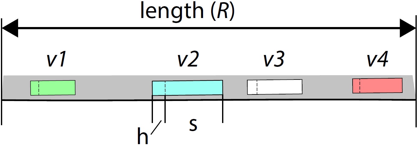
The result for L(R,t) is within the interval [0, 1], where the lower limit represents a situation with a completely free segment. The upper limit means total standstill, since this is the only case where the minimum space headway can be reached in common longitudinal models (Treiber & Kesting, 2013). Figure 1 depicts an example of a road segment where four vehicles v1 to v4 are currently driving through. The coloured areas mark the lengths required by each vehicle, including the length s of the vehicle and the specific minimum headway h, separated by a dashed line (highlighted for vehicle v2), as defined in the respective longitudinal model.

Figure 1. Single road segment containing vehicles with specific length s and headway h

As the parameter t in equation (2) indicates, the calculated load is a snapshot at a specific time. To a greater degree, the goal is to provide statistics for a longer time period , which is calculated by an averaging function over time, according to equation (3), representing a simple moving average (SMA), or equation (4), representing an exponential moving average (EMA) function. The latter provides higher weights for more recent values and is also referred to as the exponentially weighted moving average, where m represents the weighting multiplier, index j denotes the current time index, and EMA_Δt represents the current average value for the whole observation interval Δt (consisting of S values). S denotes the number of time steps under observation. The resolution r can be defined arbitrarily in real-world observations or for time-continuous simulators. In simulation environments, however, time-discrete simulators in a microscopic manner are more popular, which simplifies the selection of r, since the time step size of the simulation can be chosen.

With equation (3), we have the load statistics over the time interval Δt for a specific road segment R. When observing or simulating vehicular road traffic, a common use case is to have a larger road network region of interest, naturally consisting of multiple road segments and intersections. The simplest solution to calculate a load L(N, Δt) for this network part (denoted as N) is again to average the gained load values L(R, Δt) over the total number of road segments n, weighted by their length, as equation (7) elucidates:

By that means, a full load for a defined extract of a road network can be calculated for a specific time interval. For some applications this may be sufficient, and thus can be applied without hesitation. The problem is that L(N, Δt) tends to become more and more meaningless to a certain degree when investigating the effects of a specific action between individual observations. One could consider the variations between several days as several observations in the case of real environments, or likewise multiple simulation runs in the case of simulation environments. In each observation, the traffic density or load may be distinct. This is especially the case if the extract of the road network to consider for this calculation differs between single observations: i.e., some of the road segments are not used by any driver for a longer time in one observation, while this does not happen in another one. In other words, this happens especially when the observed properties are subject to influence by the network load and the routes of the vehicles are variable, which is true for all kinds of investigations concerning intelligent routing, dynamic route calculation and other intelligent traffic management strategies. One solution could be to select only those road segments which are used by any vehicle at any time. But, then, a single vehicle using a specific route in one observation that does not do so in the next observation would influence the network load at each time step, and hence of course also the overall result. For this reason, road segments which are unused at least during part of the observation time should be considered only temporarily (as described in the next subsection) when calculating the network load.

Time-dynamic selection of area of interest

In order to diminish the problems connected with consideration of a static selection of road segments, the segments which are included in the calculation are selected based upon their utilization. A road segment is only considered for calculation of the network load L(N, Î”t) if the inequality L(R, t) > 0 is satisfied. If a specific road segment is not considered, i.e. becomes inactive, of course its length is also not considered any more in equation (7). Mathematically expressed, a road segment is not considered if the number of vehicles on it is equal to 0 for at least the time period Δt, consisting of S intervals (see equations (3) to (5)).

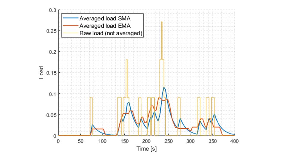
Figure 2. Load by application of simple and exponential moving averages for a single road segment

Figure 2 reveals the difference between SMA and EMA averaging for a single road segment and a total moving average length of 30 seconds. The different weighting of events become obvious therein, e.g. when focusing at second 72. The first vehicle enters the Road Segment (RS) and leaves at second 77, which causes a greater gradient for the EMA curve, which exponentially decreases in contrast to the SMA method, where the resulting average stays at a constant level for the time of the averaging interval. What is essential here is the fact that a single road segment disappears from the overall average as its particular load function result drops down to zero. Thus, it is irrelevant for the overall load quantification value for the unused periods in time.

Subsequently, this process is applied to all road segments and further leads to a single quantification value of the network load at each time interval and, according to equation (7), also for the whole observed network region. Depending on the needs of the application, the model self-evidently can be parameterized with different averaging lengths, and of course also with an arbitrary averaging method.

Evaluation by Microscopic Traffic Simulations

Undoubtedly, real-world experiments in the field of vehicular traffic with numerous involved vehicles are very costly, if not impossible, and definitely would exceed the budget of our research project. As already mentioned earlier, the cloud service which calculates the traffic load is independent of the source of information. In other words, it is irrelevant whether the data is provided by sensors of vehicles that are currently on the road and transmitted via V2X communication or by a microscopic traffic simulator. Therefore, we selected an example dealing with traffic optimization by intelligent vehicle rerouting in a microscopic simulation environment in order to demonstrate the practical applicability of the introduced methodology. The applied traffic optimization algorithm is introduced in one of our previous publications (Backfrieder, Ostermayer & Mecklenbräuker, 2017) and presents an approach to relieve congestion by traffic jam predictions, called Predictive Congestion Minimization in combination with an A*-based Router (PCMA*). Affected vehicles can then be rerouted by assigning alternative routes with free space in a timely manner and thus bypass congestion, which is proven by simulations with the microscopic traffic simulator, TraffSim (Backfrieder, Ostermayer & Mecklenbräuker, 2014). The performance of PCMA* is strongly dependent on the traffic density as well. Currently, it quantifies the traffic density by a combination of the overall number of simulated vehicles and the vehicle Inter-Arrival Interval (IAI), i.e. the static time interval between the trip start of two consecutively starting vehicles. The performance of PCMA* is measured by average travel time per vehicle, assuming all vehicles have defined immutable origin and destination locations. The system has the freedom of dynamically assigning the routes. This, of course, leads to a different utilization of the road network when the algorithm is enabled, compared to a situation with no rerouting; and also with variations depending on the selected inter-arrival interval and vehicle volume. Some road segments may be used in one configuration while they are unused in a different one, due to the dynamic route assignment. In the following analysis, we evaluate to what degree the presented methodology is representative of the network load, in place of the combination of total vehicle volume and IAI, which is more circumstantial and difficult to relate to each other.

The first hypothesis under investigation is that the network load is assumed to decrease after enabling the intelligent routing mechanism. While this seems obvious, it is also relevant to what degree the load decreases and its correlation with the figure of merit in Backfrieder, Ostermayer & Mecklenbräuker (2017), which evaluates (among other things) the performance in travel time. Subsequently, the second hypothesis claims that the network load needs to drop in a similar manner to the observed average travel time of each vehicle, since the only possibility for improvements for the PCMA* routing approach is to distribute vehicles’ routes differently compared to the original routes. We admit that this correlation is a strong simplification, but it still turns out to be fundamentally correct. Figure 6 indicates the correlation between traffic load (as a single value for a whole and highly dynamic traffic simulation) and average vehicle travel time.

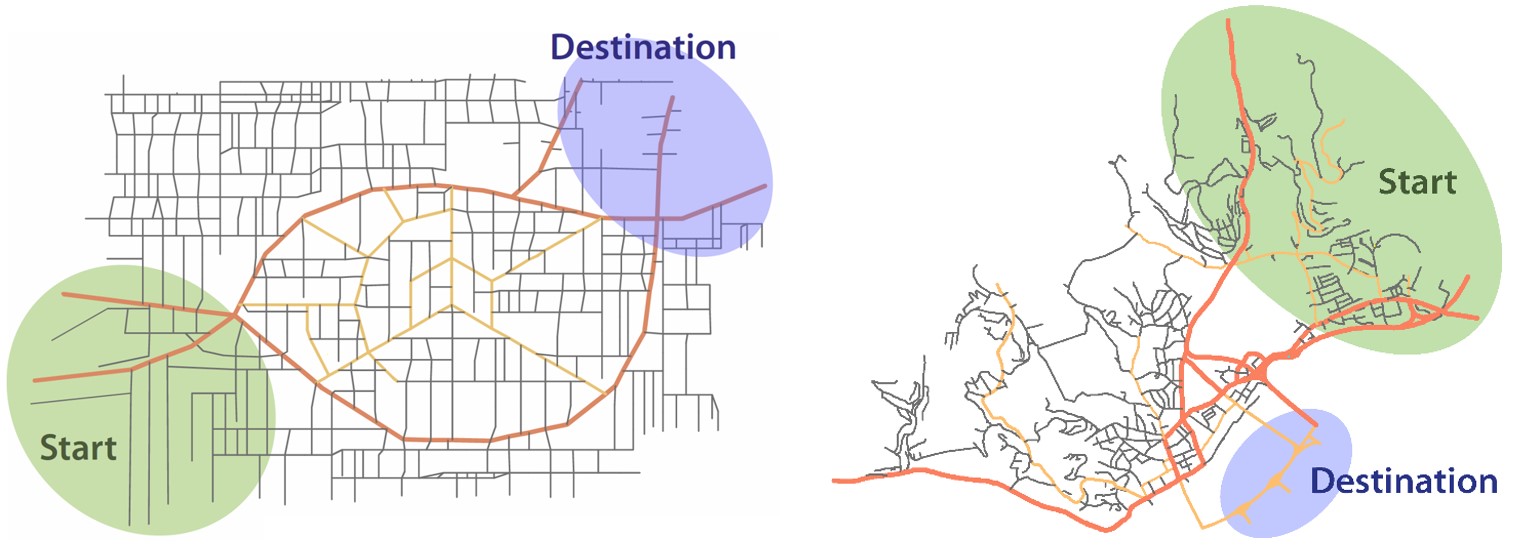
We therefore also use the traffic simulator TraffSim, configured as defined in Backfrieder, Ostermayer & Mecklenbräuker (2017) in order to gain meaningful and comparable perceptions. Two different road networks (scenarios) are under consideration. One is an artificially designed network (Figure 3 left) and the other one is a real-world scenario from the city of Linz (Figure 3 right). All vehicles start within the green ellipse and travel towards the blue destination area, which is intended to somehow represent commuters travelling to their workplace within the city. Furthermore, in the artificial scenario, the low-level roads are rarely used, whereas, in the Linz scenario, the western part of the map is rarely used or even unused. These facts elicit the need for a dynamic consideration of the road infrastructure, as explained previously in the related work section.

Figure 3. Investigated road network scenarios (left: artificial street network, right: City of Linz, Austria)

Evaluation of achieved average travel time vs traffic load

Initially, we compare the achieved average travel time with the calculated traffic load of the very same simulation run. As explained earlier, the average vehicle travel time depends on both the total number of simulated vehicles and the IAI. The evaluation is done for two configurations, which represent a non-optimized and an optimized setup. We use the SMA method with averaging length 30 seconds. Note that we only show results for these parameters, since the behaviour is very similar when setting the parameters to different values.

Setup with disabled traffic optimization

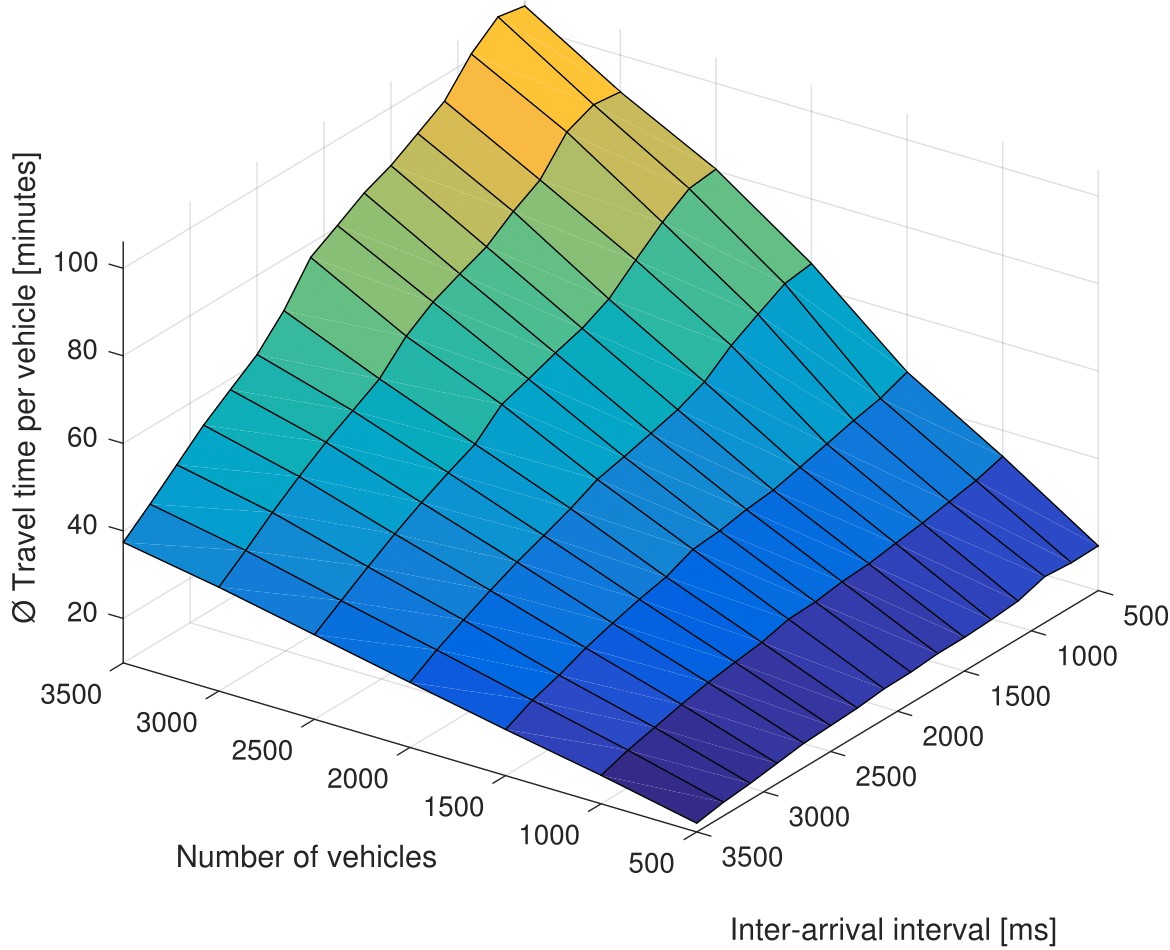
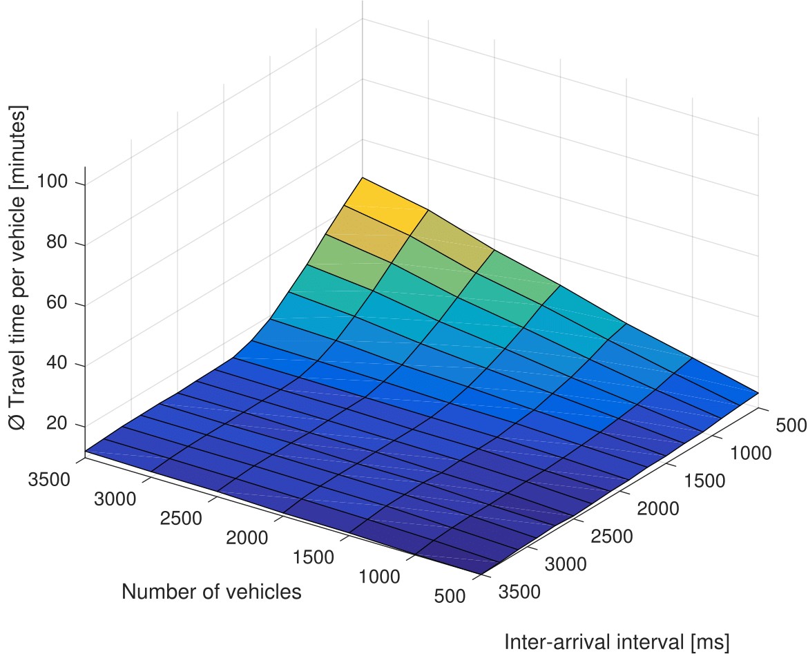
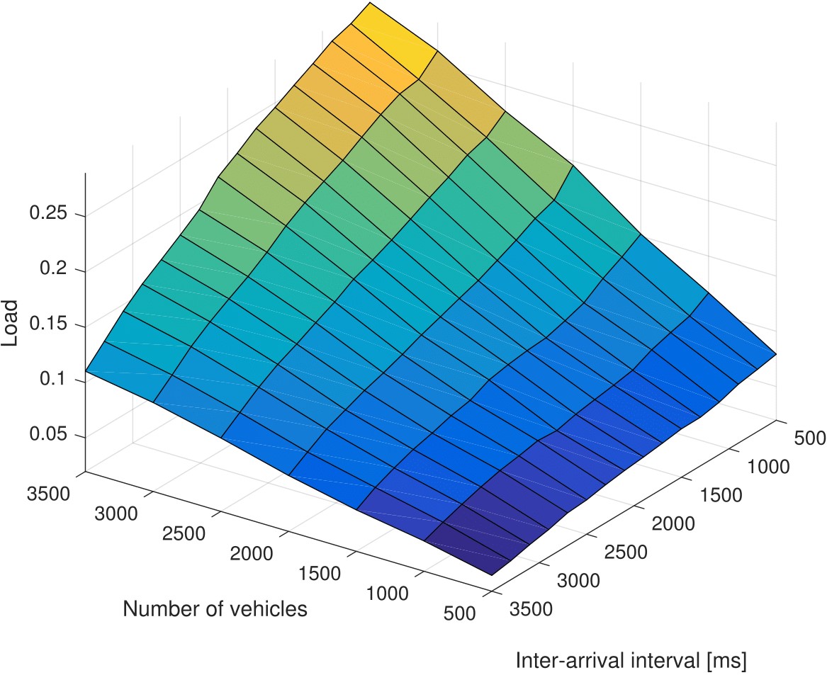
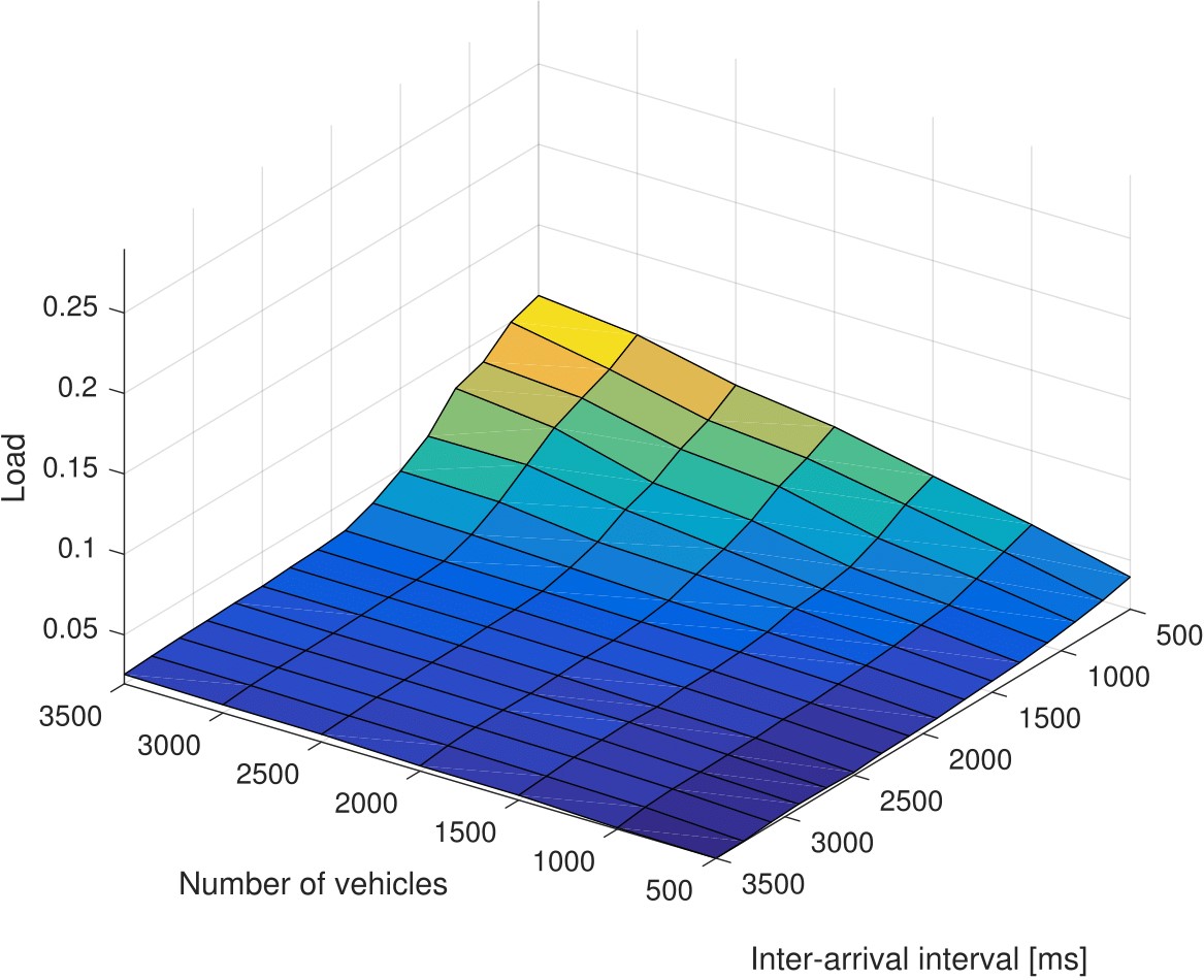
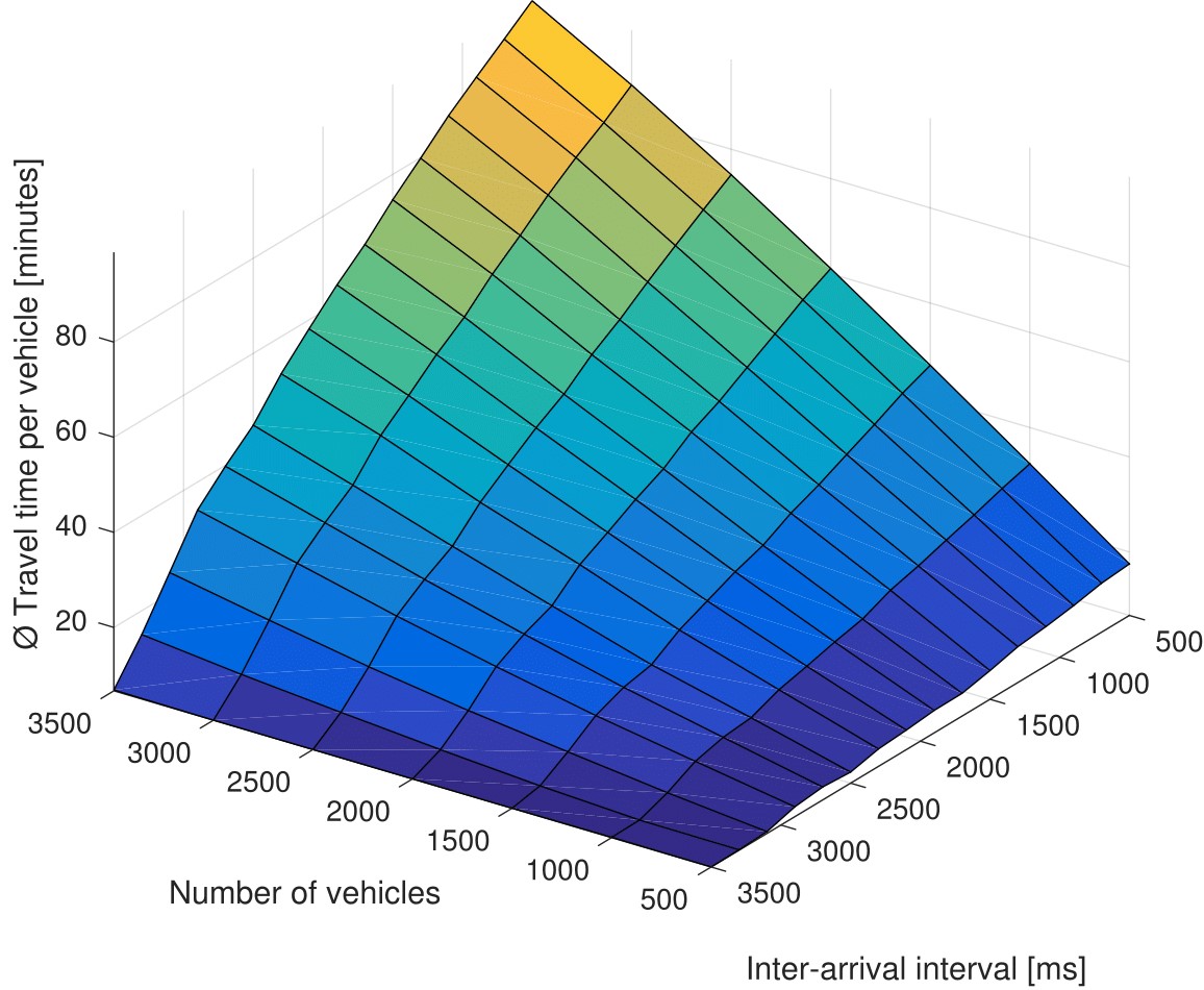
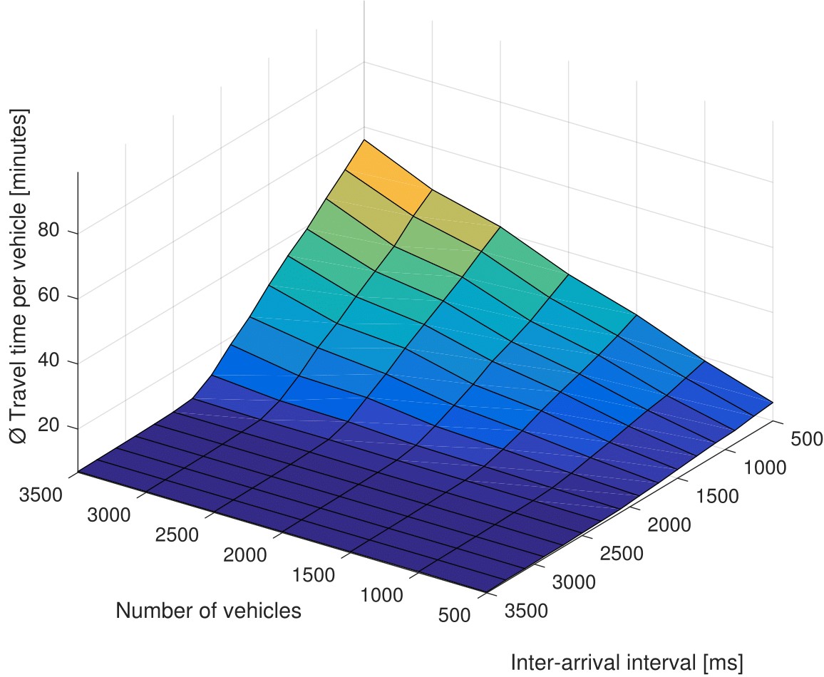
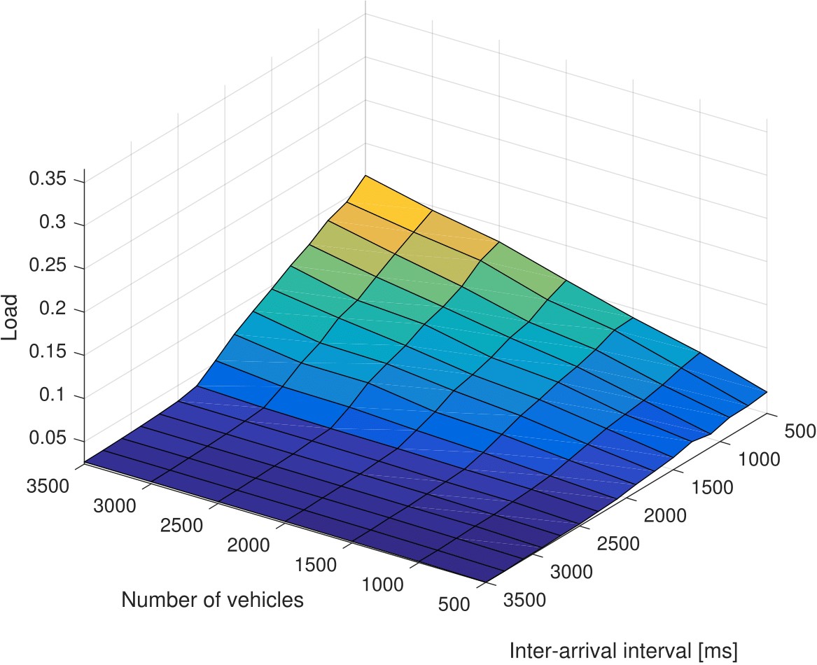
First, the traffic load is calculated in a situation where traffic optimization is disabled, i.e. no route advice is provided for any vehicle and all of them choose the shortest route, independent of any emerging traffic jams. Figures 4a and 5a show the achieved average travel time vs IAI and overall vehicle amount, while Figures 4c and 5c depict the resulting load as defined in equation (7). What becomes obvious here is that the figure pairs 4a/4c and 5a/5c reveal a very similar shape. Both have their peak in the back upper corner, where arrival intervals are short and the number of vehicles is high. However, what also can be extracted from these figure pairs is the fact that there exist different combinations of IAI and vehicle volume that lead to the same load and very similar performance in terms of average travel time. This is one big benefit of quantifying the load in a general manner instead of the dependence on vehicle volume and arrival interval.

Figure 4. Average vehicle travel time and load without (a, c) and with (b, d) intelligent traffic optimization (artificial scenario)

Despite the general similarity of the surfaces, in the Linz scenario (Figure 5) there is still a slight difference visible when comparing the two shapes. Figure 5a has a more linear gradient when looking backwards (i.e. lower IAI and higher vehicle amount), while Figure 5c is more belly-shaped with medium x- and y-values. This can be explained by long traffic jams that occur due to the heavy overload of the road network, which disappear very slowly and dramatically increase the travel time of the vehicles. In this scenario a large share of the entire road network is congested. The travel time therefore comparatively is much higher, while the load still does not increase any more if all used roads are jammed. In the artificial scenario this behaviour does not occur, since the chosen combinations of the parameters “number of vehicles” and “IAI” fit better to the capacity of the road network, meaning that a large part of the network is not congested. This leads to the fact that the shapes of the surfaces in Figures 4a and 4c are very similar.

Figure 5. Average vehicle travel time and load without (a, c) and with (b, d) intelligent traffic optimization (Linz scenario)

Setup with enabled traffic optimization

In the second setup, the best performing setup of PCMA* is chosen (according to Backfrieder, Ostermayer & Mecklenbräuker (2017)) in order to evaluate how the calculated traffic load correlates with the average vehicle travel time if dynamic rerouting is enabled. Figures 4 (artificial scenario) and 5 (Linz scenario) show the achieved average vehicle travel time (Figures 4b and 5b, respectively) in contrast to the calculated load (Figures 4d and 5d, respectively). In the artificial scenario the surfaces are still very close to each other, whereas in the Linz scenario they are much closer to each other than before, which reveals the fact that the optimized average vehicle travel time is directly proportional to the configured traffic load for a wide range of parameter combinations of IAI and number of vehicles. The next subsection clarifies the relation between the two surfaces in more detail.

Comparison of normalized traffic load and travel time

In order to point out the correlation between the calculated load and the achieved average vehicle travel time of the optimization, we calculate the fraction of the average vehicle travel time TT(Δt) and the respective calculated load L(N, Δt) as the proportionality factor k_TT,L:

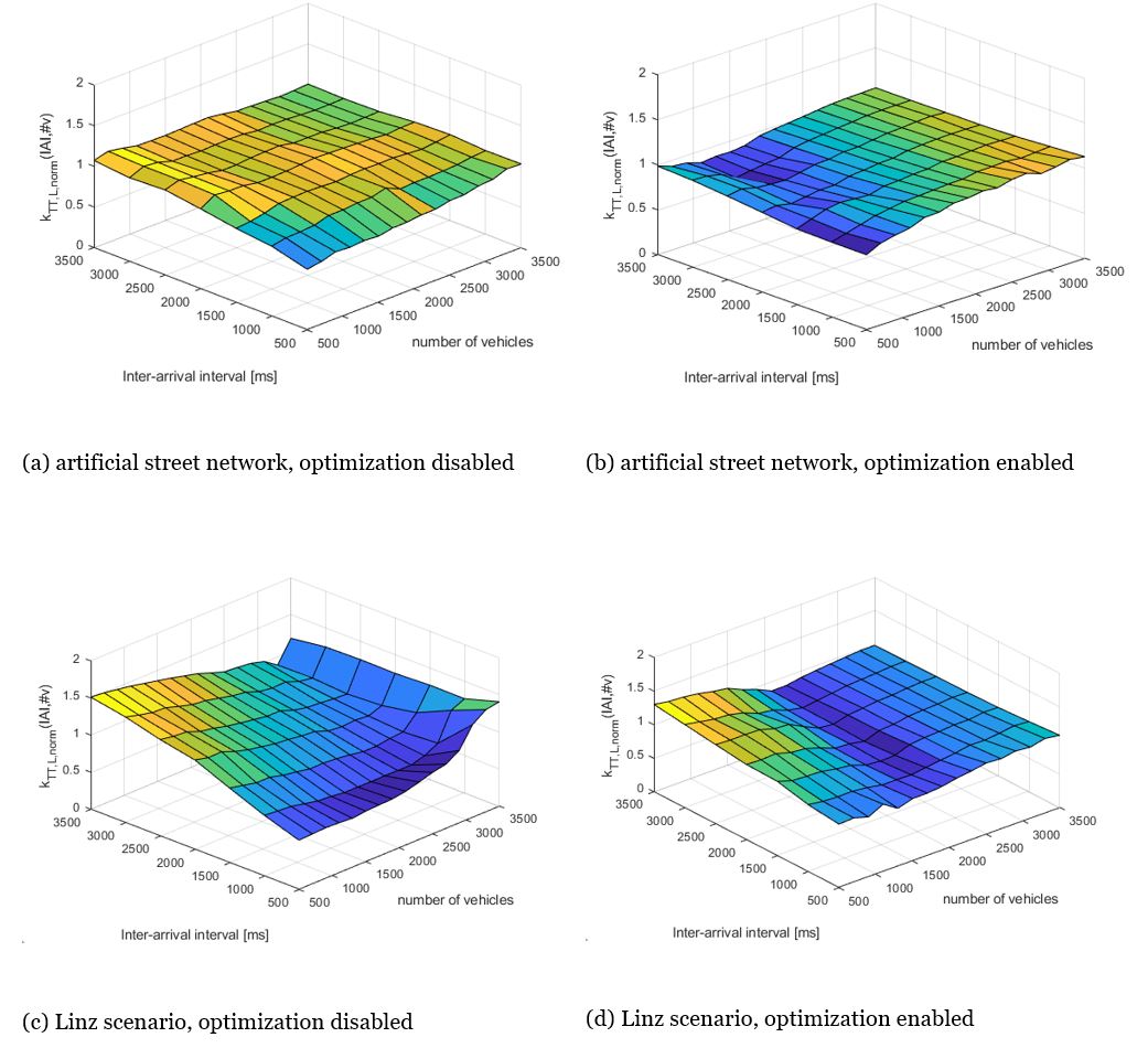
This value is normalized to its mean value and results in the normalized proportionality factor k_TT,L,norm. Figure 6 shows k_TT,L,norm for different parameter pairs IAI and number of vehicles and Δt as the time for a whole simulation run of 3000 vehicles.

Basically, a surface parallel to the IAI/number-of-vehicles plane means a constant proportionality factor k_TT,L,norm for the entire parameter pair range. This means that the mapping from load to average vehicle travel time can be done for the entire parameter range with the knowledge of k_TT,L for a single parameter pair. Usually there is a dependency on the parameters IAI and number of vehicles (#v) leading to k_TT,L(IAI, #v) and k_TT,L,norm(IAI, #v), respectively.

One can see that enabling the traffic optimization algorithm (Figure 6 right) has an impact on the proportionality factor. This is because the optimization algorithm helps to distribute the traffic over a higher number of road segments, leading to fewer traffic jams. A quite high dependency of k_TT,L,norm on IAI and #v can be observed in Figure 6c. The reason for that was already explained in the two previous sections. Introducing the traffic optimization algorithm reduces the dependency of k_TT,L,norm on IAI and #v.

What we can see is that there is a dependency on both road network and application of traffic optimization algorithms. Note that the proportionality factor k_TT,L is almost constant in case of not too heavy traffic jams, whereas, in the other case, the proportionality between load and average vehicle travel time gets more dependent on the selected parameter pair and a single proportionality factor for the entire parameter pair range loses validity. Comparing Figures 6c and 6d shows that the application of the traffic optimization algorithm flattens the surface in the range of heavy traffic (small IAI and high number of vehicles) due to its ability to distribute the traffic over more street segments, avoiding heavy traffic jams. But there still remains an increase of k_TT,L,norm in the case of low traffic (high IAI and low number of vehicles). We expect that low traffic density leads to higher traffic flow, causing higher average speeds of the vehicles. In that case, the headway of the vehicles increases for safe driving. Since in our metric this headway is constant, the load is underestimated, leading to an increase of the proportionality factor. A consideration of this issue is a task for future work.

Figure 6. Normalized proportionality factor k_TT,L,norm(N,Δt) between load and average vehicle travel time without (a, c) and with (b, d) intelligent traffic optimization in the artificial road network scenario (top) and the Linz scenario (bottom)

Summary and Conclusions

We have proposed a novel methodology to quantify the traffic load over time, with special focus on scenarios where the usage of road space is dynamic and varies over time. Our approach is able to determine the traffic load of an extract of the road network during a specific time period, but also to calculate a single load quantification number. For the latter, it is necessary to focus on the parts of the road that are actually used, instead of always taking into account a predefined part of the road network as done by related research in this field. In order to achieve this, we introduce two possibilities to eliminate distortions of the traffic load.

The proposed methodology is implemented as a cloud service, which requires location information in short time intervals to work precisely. The current positions of the vehicles are transmitted to the cloud at regular time intervals by V2I communication. However, this implies that all vehicles are somehow able to report the required data via wireless communication; otherwise the calculated numbers will underestimate the actual conditions on the road.

We demonstrate the applicability of the presented methodology by simulations, which compare the performance of PCMA*, a predictive rerouting and traffic optimization approach from the literature, to the calculated traffic load. As the only possibility for the dynamic re-router is to make use of additional, previously unused road space, the traffic load is assumed to decrease and correlates well with the achieved optimization performance (average vehicle travel time). The results of this comparison show very good proportionality between the calculated traffic load quantification and the achieved optimized average travel time in the artificial road network case and an acceptable proportionality for the Linz scenario.

In the end, this paper introduces a novel methodology to quantify the traffic load statistic for a defined road network extract and over a defined time period by a single number between 0 and 1, which is also a (very) good indicator of the achievable average vehicle travel time. It is much easier to apply than comparable approaches, and still adjustable to fulfil an individual application’s needs.

Acknowledgements

This project has been co-financed by the European Union using financial means of the European Regional Development Fund (EFRE). Further information on IWB/EFRE is available at https://www.efre.gv.at.

References

Abadi, A., Rajabioun, T., Ioannou, P. A. (2015). Traffic Flow Prediction for Road Transportation Networks with Limited Traffic Data. IEEE Transactions on Intelligent Transportation Systems, 16(2), 653–662.

Abbas, T., Sjöberg, K., Karedal, J., Tufvesson, F. (2015). A Measurement Based Shadow Fading Model for Vehicle-to-Vehicle Network Simulations. International Journal of Antennas and Propagation, 2015, 1-12. DOI: 10.1155/2015/190607

An, X., Hou, Q., Li, N., Zhai, S. (2013). Assessment of Human Exposure Level to PM10 in China. Atmospheric Environment, 70, 376–386.

Athol, P. (1965). Interdependence of Certain Operational Characteristics within a Moving Traffic Stream. Highway Research Record, 72, 58–87.

Aw, A., Rascle, M. (2000). Resurrection of “Second Order” Models of Traffic Flow. SIAM Journal on Applied Mathematics, 60(3), 916–938.

Backfrieder, C., Ostermayer, G., Mecklenbräuker, C. F. (2014). TraffSim – A Traffic Simulator for Investigations of Congestion Minimization through Dynamic Vehicle Rerouting. International Journal of Simulation – Systems, Science and Technology, 15(4), 38–47.

Backfrieder, C., Ostermayer, G., Mecklenbräuker, C. F. (2017). Increased Traffic Flow through Node-based Bottleneck Prediction and V2X Communication. IEEE Transactions on Intelligent Transportation Systems, 18(2), 349–363.

Backfrieder, C., Lindorfer, M., Mecklenbräuker, C. F., Ostermayer, G. (2018). Robustness of Intelligent Vehicular Rerouting towards Non-ideal Communication Delay. Proceedings of the Future of Information and Communication Conference, 143-164, Singapore.

Behrisch, M., Bieker, L., Erdmann, J., Krajzewicz, D. (2011). SUMO - Simulation of Urban MObility - an Overview. Proceedings of the 3^rd International Conference on Advances in System Simulation, 55–60, Barcelona, Spain.

Blazek, T., Backfrieder, C., Mecklenbräuker, C. F., Ostermayer, G. (2017). Improving Communication Reliability in Intelligent Transport Systems through Cooperative Driving. Proceedings of the 10th IFIP Wireless and Mobile Networking Conference, 1-6, Valencia, Spain.

Boskovich, S., Barth, M. (2013). Vehicular network Rerouting Autonomy with a V2V, I2V, and V2I Communication Matrix Classification. Proceedings of the 16^th International IEEE Conference on Intelligent Transportation Systems, 172-177, The Hague, Netherlands.

Cassidy, M., Coifman, B. (1997). Relation among Average Speed, Flow, and Density and Analogous Relation between Density and Occupancy. Transportation Research Record: Journal of the Transportation Research Board, 1591, 1–6.

Cappiello, A., Chabini, I., Nam, E. K., Lue, A., Zeid, M. A. (2002). A Statistical Model of Vehicle Emissions and Fuel Consumption. Proceedings of the 5th IEEE International Conference on Intelligent Transportation Systems, 801–809, Singapore.

Chan, K. Y., Dillon, T., Chang, E. (2013). An Intelligent Particle Swarm Optimization for Short-term Traffic Flow Forecasting Using on-road Sensor Systems. IEEE Transactions on Industrial Electronics, 60 (10), 4714–4725.

Chen, A., Subprasom, K., Ji, Z. (2006). A Simulation-based Multi-objective Genetic Algorithm (SMOGA) Procedure for BOT Network Design Problem. Optimization and Engineering, 7(3), 225–247.

Elbery, A., Rakha, H., Elnainay, M., Drira, W., Filali, F. (2015). Eco-Routing Using V2I Communication: System Evaluation. Proceedings of the 18th IEEE International Conference on Intelligent Transportation Systems, 71–76, Las Palmas, Spain.

Gazis, D. C., Edie, L. C. (1968). Traffic Flow Theory. Proceedings of the IEEE, 56(4), 458–471.

Greenshields, B. D. (1935). A Study of Traffic Capacity. Highway Research Board, 14, 448-477.

Hoogendoorn, S. P., Bovy, P. H. (2001). State-of-the-art of vehicular traffic flow modelling. Proceedings of the Institution of Mechanical Engineers, Part I: Journal of Systems and Control Engineering, 215, 283-303.

Horvitz, E. J., Apacible, J., Sarin, R, Liao, L. (2009). Prediction, Expectation, and Surprise: Methods, Designs, and Study of a Deployed Traffic Forecasting Service. arXiv:1207.1352 [physics], 2012. [Online]. Available: http://arxiv.org/abs/1207.1352

Jing, B., Wu, L., Mao, H., Gong, S., He, J., Zou, C., Song, G., Li, X., Wu, Z. (2016). Development of a Vehicle Emission Inventory with High Temporal Spatial Resolution based on NRT Traffic Data and its Impact on Air Pollution in Beijing Part 1: Development and Evaluation of Vehicle Emission Inventory. Atmospheric Chemistry and Physics, 16(5), 3161–3170.

Kumar, R., Chhabra, S. (2016). Efficient Routing in Vehicular Ad-hoc Networks Using Firefly Optimization. Proceedings of the 2016 International Conference on Inventive Computation Technologies, 1–6, Coimbatore, India.

Lighthill, M. J., Whitham, G. B. (1955). On Kinematic Waves. I. Flood Movement in Long Rivers. Proceedings of the Royal Society of London. Series A, Mathematical and Physical Sciences, 281–316.

Lindorfer, M., Mecklenbräuker, C. F., Ostermayer, G. (2017). Modeling the Imperfect Driver: Incorporating Human Factors in a Microscopic Traffic Model. IEEE Transactions on Intelligent Transportation Systems, 19(9), 2856–2870.

Mandziuk, J., Swiechovski, M. (2016). Simulation-based approach to Vehicle Routing Problem with Traffic Jams. Proceedings of IEEE Symposium Series on Computational Intelligence, 1-8, Athens, Greece.

Nafi, N., Khan, R., Khan, J., Gregory M. (2014). A Predictive Road Traffic Management System based on Vehicular Ad-hoc Network. Proceedings of the International Telecommunication Networks and Applications Conference, 135-140, Melbourne, Australia.

Nebbou, T., Fouchal, H., Lehsaini, M. (2017). Metrics for Vehicle Density in Urban Environment. Proceedings of the 2017 IEEE Global Communications Conference, 1–6, Singapore.

Ni, D. (2015). Traffic Flow Theory: Characteristics, Experimental Methods, and Numerical Techniques. Butterworth-Heinemann.

Pan, J., Khan, M., Sandu Popa, I., Zeitouni, K., Borcea, C. (2012). Proactive Vehicle Re-routing Strategies for Congestion Avoidance. Proceedings of the 8th IEEE International Conference on Distributed Computing in Sensor Systems, 265–272, Hangzhou, China.

Stevanovic, A., Stevanovic, J., Zhang, K., Batterman, S. (2009). Optimizing Traffic Control to Reduce Fuel Consumption and Vehicular Emissions: Integrated Approach with VISSIM, CMEM, and VISGAOST. Transportation Research Record: Journal of the Transportation Research Board, 2128, 105–113.

Szeto, W. Y., Jiang, Y., Wang, D. Z. W., Sumalee, A. (2015). A Sustainable Road Network Design Problem with Land Use Transportation Interaction Over Time. Networks and Spatial Economics, 15(3), 791–822.

Treiber, M., Kesting, A. (2013). Traffic Flow Dynamics. Berlin, Heidelberg. Springer.

Zhang, B., Ma, M., Liu, C., Shu, Y. (2017). Delay Guaranteed MDP Scheduling Scheme for HCCA based on 802.11p Protocol in V2R Environments. International Journal of Communication Systems, 30(15), 1-12.

Zhou, X., Tanvir, S., Lei, H., Taylor, J., Liu, B., Rouphail, N. M., Frey, H. C. (2015). Integrating a Simplified Emission Estimation Model and Mesoscopic Dynamic Traffic Simulator to Efficiently Evaluate Emission Impacts of Traffic Management Strategies. Transportation Research Part D: Transport and Environment, 37, 123–136.